- za 10 maart 2018
- education
- Jason K. Moore, Kenneth Lyons
- #education, #engineering, #python, #jupyter, #computational thinking
Co-authored by co-instructors Jason K. Moore and Kenneth Lyons.
Course Description
Introduction to Mechanical Vibrations is a 30+ year old upper level elective in the mechanical engineering curriculum at the University of California, Davis. It is a classic mechanical engineering course that stems from the courses and books of Timoshenko and Den Hartog from the early 20th century. The course advances students' understanding of vibrating mechanical systems, that has a foundation is the theory of small periodic motions resulting from the mathematical analysis of linear differential equations derived from Newton's Second Law of Motion. These foundational concepts provide insight into the design of machines to both minimize undesired vibrations and exploit desired vibrations.
Animation of a car vibration model created with resonance; an example of the type of systems students analyze and design in the course.
Most mechanical vibration courses have been presented primarily from a theoretical perspective which was tied to the early analytic tools. There have also been some courses with accompanying laboratories to experiment with real vibrating systems, but those are fewer and far between. Also, since the late 80s, mechanical vibrations courses have often been enhanced with computational tools, such as Matlab, to solve problems that are difficult or unwieldy to solve by hand.
These courses typically have the standard engineering course format, i.e. the professor lectures in class by deriving mathematical theory on the board and does example problems to accompany the theory, the students are assigned homework problems each week for practice at applying and understanding the theory, and exams are given that are similar to homework problems to assess student learning.
This format has served the engineering profession well for a century or more, but there are a number of reasons to believe that this course could be changed to both improve learning and provide students with skills that are more relevant to their future work.
Why Change?
The main reasons that we wanted to change the course are that:
- This type of course has likely only changed in one significant way in the past century with addition of accessible computational tools in the 80s. Although it is true that the foundational theory has not changed much in that time, much of the traditional material may not be directly relevant to solving modern vibration related problems and thus could be removed.
- Traditional engineering textbooks are becoming antiquated due to their high cost to the students, their scope not being well-suited to the courses they are designed for, the fact that they are closed access, and that they do not utilize the power of the world wide web to optimally enhance the materials. Additionally, there is a long list of mechanical vibrations textbooks and editions from the past 100 years that more-or-less provide the same materials.
- There is evidence that methods other than the traditional lecture style of typical engineering classes are more effective for student learning. Many of these "learn by doing" methods align extremely well with engineering.
- We would like to increase the likelihood that students utilize "computational thinking" and the related tools to solve engineering problems when they leave our bachelor's program.
Computational Thinking
The last point above requires some elaboration, as it is a central tenant to the course redesign. Engineering courses often have computational components, but students may or may not learn to "think computationally."
An engineer's primary goal is to solve problems, using the knowledge and tools at hand. Solving each problem requires some understanding of how the world works. Engineers perform experiments and develop mathematical models of the phenomena they observe in order to make predictions about similar phenomena. Thus, it is well known that if one could reason about the world using mathematical language, one could gain great power to change it. With the advent of computers, computation has typically been used to enhance the mathematics so that mathematical problems could be solved more efficiently. Mostly, math is translated into computer code. The steps are something along the lines of:
- Observe phenomena
- Optionally, perform a controlled physical experiment to learn specifically about the phenomena
- Develop a mathematical, causal relationship that predicts the phenomena
- Implement the mathematical model computationally
- Use the computational model to make predictions and solve problems
This is a powerful and invaluable process, but it is also interesting that, taken to an extreme, one may be able to remove step 3 and reason about the world in the language of computation directly.
An example
Calculating probabilities offers simple examples that can highlight what we mean. For example, if you want to answer:
What is the probability of rolling at least two 3's if you roll a 6-sided die 10 times?
A mathematician or statistician is likely to formulate the following equation using probability theory:
and when you complete the numerical calculation you will find the probability is about 52 in a 100. To be able to do this you need to be well versed in a number of mathematical concepts that are often abstract relative to the primary question such as probability distributions, conditional probability, the binomial theorem, factorials, etc.
From an experimentalist's perspective, you can also literally roll 10 dice many many times and tally how many of the sets of rolls met the criteria. Thinking about this experiment is much easier than reasoning about probabilities, and many of the abstractions are removed. However, you'd have to roll the ten dice upwards of 10000 times to get an accurate estimate of the probability. Fortunately, this is something a computer is good at. Being able to reason about this problem and, for example, write the following Python code, you will get the same answer as reasoning through probability theory. In this case, computational reasoning is likely vastly simpler than what is needed for the mathematical reasoning if you have basic programming concepts in your toolbox.
from random import choice
num_trials = 10000
dice_sides = [1, 2, 3, 4, 5, 6]
count = 0
for trial in range(num_trials):
    ten_rolls = [choice(dice_sides) for roll in range(10)]
    if ten_rolls.count(3) > 1:
         count += 1
print(count / num_trials)
The required knowledge here spans variables, data structures, loops, and flow control but it has the advantage that it maps directly to the experimental process with very little abstraction. Additionally, this knowledge is used in every computational problem, not just ones about probability.
This ability to reason about the world through computational language is a prime of example "computational thinking." Computational thinking adds a complementary mode of reasoning to experimentation and mathematical modeling. In some cases, it may even be used as a replacement for one, the other, or both.
So this raises the question: "If we drastically increase the focus on computational thinking to learn about mechanical vibrations, will students be better equipped to solve real vibration problems when they leave the class?" We believe they will, but there are a number of aspects that needed to be changed in the course to do test this.
What We Did
The course redesign required quite a number of changes in order to structure the learning around computational thinking and meet the other goals. The following presents summaries of the various changes and activities we did to bring this to fruition:
Interactive Open Access Digital Textbook
We wrote a series of 14 modules in the form of Jupyter notebooks that serve as the core learning resources for the course. We consider these notebooks, taken together, as a textbook that replaces the need for a traditional static, paper text. The design of this text has these features:
- Approximately 1 notebook for each of the 20 two hour lecture periods, i.e. just the right length for the 10 week course.
- The notebooks mix written text, mathematical equations, static figures, videos, and live Python code that can be executed to create interactive figures.
- Each notebook introduces a new real (and hopefully interesting) vibrating mechanical system as a motivation for learning the subsequent concepts.
- Computational thinking approaches are utilized if possible.
- The notebooks are licensed under the Creative Commons Attribution license to maximize reuse potential.
- The notebooks are intended to be used live in class with embedded interactive exercises.
Below is a static version of one of the notebooks:
You can execute the notebooks if you load them using Binder
Software Library
The text book is accompanied by a custom Python software library called "resonance". We decided to create this library so that we could carefully design the application programming interface (API) and build up exposure to the concepts we introduced in the text. The library was designed with these features in mind:
- Provide a framework for learning mechanical vibration concepts.
- Allow students to construct, simulate, analyze, and visualize vibrating systems with a simple API.
- Hide some Python programming details up front, but allow them to be exposed through scaffolding as the course progresses.
- Hide object oriented class construction completely.
- Include many and appropriately informative error messages.
- Performance is secondary to usability and learning.
- Structured around "system" objects that have similarities to real vibrating mechanical systems and can be experimented with similarly to how one would experiment with a physical apparatus in a lab.
Below shows a quick example of how the library would be used to construct and simulate a linear model of simple pendulum:
from resonance.linear_systems import SingleDoFLinearSystem

# create a system
sys = SingleDoFLinearSystem()

# define the constant parameters
sys.constants['length'] = 1.0  # m
sys.constants['grav_acc'] = 9.8  # m/s

# define the coordinate and its derivatives
sys.coordinates['angle'] = 0.1  # rad
sys.speeds['ang_rate'] = 0.0  # rad/s

# define a function that returns the coefficients of the canonical
# differential equation: m x'' + c x' + k x = 0
def coeff_func(length, grav_acc):
    """Returns m, c, k."""
    return 1.0, 0.0, grav_acc / length

sys.coeff_func = coeff_func

# simulate the system for 5 seconds given the initial values
traj = sys.free_response(5.0)

# print the array of angle values
print(traj.angle)
Active Computing In Class
The notebooks were presented live in class and followed a similar style to the Software Carpentry method of teaching computational skills. Each student downloaded the notebook at the beginning of the class period for use on their laptop. The instructor led the students through the notebooks by offering verbal summaries and addenda to the written text via "board work." The instructor executed the code cells to produce various figures and then discussed them, often live coding answers to questions. Each notebook included short exercises (about 5-8 per 2 hr period) interspersed throughout the text that were geared to assessing students on the prior 10 minutes of instruction and reading. These exercises had easily accessible solutions to ensure students could move forward even if the solution was not obtained in the allocated time. We attempted to pace the exercises such that the vast majority of the class completed them before moving forward. The students were encouraged to work together and the instructors were present to answer questions during the exercises. The notebooks were submitted at the end of the class for participation credit.
JupyterHub Service
We purchased a server and installed the cloud computing service JupyterHub for the students to use both in and out of class for their course work. This turned out to be a great idea for several reasons:
- Students did not have to install any software; we fully controlled the computation environment to ensure everything worked as desired and all students had access to this common environment without following a complex installation process.
- We were able to update the custom software library at any time. This allowed us to write the library incrementally as we created the course content. At one point, Kenny fixed a library bug live in class as soon as we uncovered it.
- We were able to utilize nbgrader for distribution, collection, and grading of the in-class materials and homework assignments (see more below).
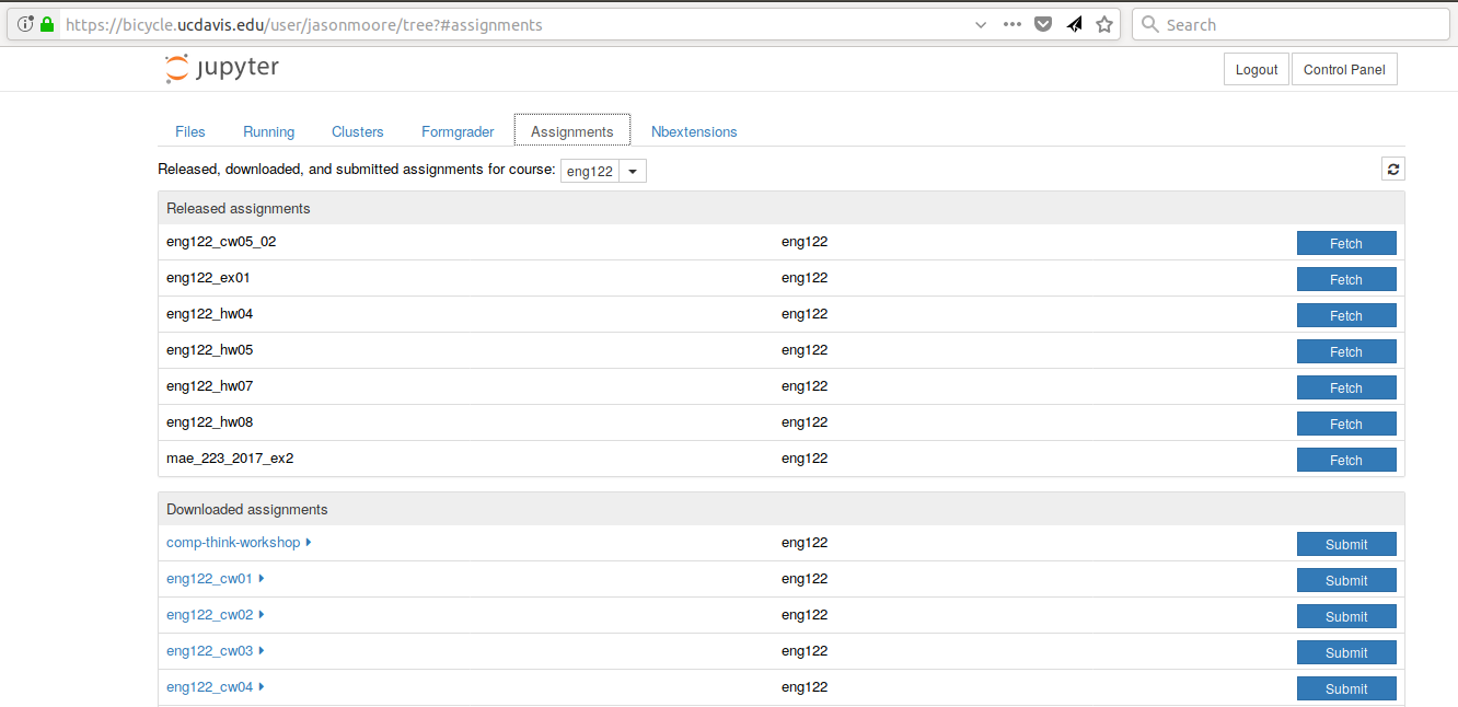
A screenshot of the Jupyterhub nbgrader interface that lets students fetch and submit assignments.
Computational Homeworks
We developed 8 homework sets to supplement classwork and to assess the students' ability to apply in-class materials to different problems. These were all implemented as Jupyter notebooks and were distributed, collected, and graded using nbgrader.
The first 3 homework notebooks were fully-formatted notebooks in which students supplied code, text, figures, and equations to predetermined sub-problems (think "fill-in-the-blanks"). One issue with this style of assessment is that it provides too much structure and emphasizes details of one approach to the problem. Since we also wanted students to be able to reason about systems at a high level of abstraction and formulate computational experiments to answer questions about them, we switched to a more open-ended format where each homework assignment included 3 or 4 problem statements and students were expected to populate the notebooks with as many cells as needed to answer the problems. This had the added benefit of giving students practice communicating their reasoning, computations, and interpretations of results.
Students were given individual feedback on their homework notebooks, and we created homework solutions to demonstrate exemplary formatting and style conventions, supplementing the in-class materials. Formatting and overall clarity of the submitted homework notebooks seemed to improve significantly by the end of the course.
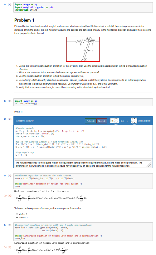
A screenshot of the nbgrader grading interface for a single homework problem.
Project Instead of Exams
The previous course design had two in-class pen-and-paper exams. We added an individual course project to more effectively assess the course learning objectives and provide a realistic engineering exercise.
We originally intended to have a midterm, a final, and a course project but we dropped the final exam due to two reasons:
- Two exams and a project was simply too much work in a 10-week course.
- We gave a midterm that required live coding to solve the problems, and this did not effectively assess what the students had learned, due to students getting caught on programming issues more than anticipated.
Next year, we will likely remove the midterm and break the project into two phases. The projects proved to be a much more effective method for students to demonstrate what they had learned.
SciPy BoF
We led a "Birds of a Feather" session on teaching modeling and simulation at SciPy 2017 in Austin, Texas. There were 13 participants from a variety of disciplines and schools. Notes from this session can be found in a separate blog post. This BoF introduced a large number best practices for teaching these types of courses and established a network of potential collaborators.
Computational Thinking Workshop and Seminar
We also wanted to share these methods with the STEM faculty at UC Davis. To do so, Allen Downey of Olin College and we held a workshop titled "Computational Thinking in the Engineering and Sciences Curriculum" at the UCD Data Science Institute on January 5th for about 20 faculty, staff, and graduate students from a variety of disciplines around campus. We proposed seven methods of utilizing computation to learn domain-specific concepts, and the attendees developed a variety of examples from courses they have taught or would like to teach. The abstract read:
This workshop invites faculty to think about computation in the context of engineering education and to design classroom experiences that develop programming skills and apply them to engineering topics. Starting from examples in signal processing and mechanics, participants will identify topics that might benefit from a computational approach and design course materials to deploy in their classes. Although our examples come from engineering, this workshop may also be of interest to faculty in the natural and social sciences as well as mathematics.
The workshop was recorded:
and the accompanying slides are available here:
In addition to the workshop, Allen gave a more general seminar on "Programming as a Way of Thinking", which can be viewed below:
along with the slides:
Also see Allen's blog post on the workshop and seminar.
What To Improve
Over the course of developing and teaching the class, we noted a number of things to adjust for a second offering. These are tracked in resonance's issue tracker. We've also had focus groups with a few students in the course to get more critical feedback of the materials and methods, which can also be found in the issue tracker. The following list provides some of the more important changes we plan to make:
- The programming skills necessary to solve the vibration problems need to ramp up more gradually. Fixing this will involve hiding more details in the software library and pacing the exposure of these details more linearly through the notebook progression.
- Some of the notebooks are too long and complicated. The notebooks need to be divided into smaller chunks that map to about 40 in-class learning sessions.
- The textbook needs to be completed such that each notebook has sufficient text to explain the lesson without the instructor explaining it.
- More of the analytical methods need to be introduced after the computational methods, especially for the concepts where the analytical methods prove to be a superior tool.
- Students balancing a laptop and notebook on a standard desk is difficult. We need a classroom that is appropriate for the class activities (i.e. need tables!).
Conclusion
After the first delivery of the course, a good question to ask may be "Can students solve problems related to mechanical vibrations better than if they were to have taken a different course?", as that is our primary objective. It was evident from their final projects that they could, but the project problem was designed by us to be solvable with the things we knew (or hoped) they'd learned. This question is difficult to answer without a properly designed and executed experiment, which may be something that should be done in the future. We have received a mix of feedback on the course that encompassed students enjoying it thoroughly to students that struggled getting past the programming requirements. It was quite fun to teach and really impressive to see the skills the students developed over the course both in vibrations and computational thinking with Python. Overall, we feel good about the course direction and will continue to improve it.
Acknowledgements
This effort was supported with funding from the Undergraduate Instructional Innovation Program, which is backed by the Association of American Universities (AAU) and Google, and administered by UC Davis's Center for Educational Effectiveness. The funding proposal can be viewed on Figshare.
We thank Allen Downey from Olin College for visiting and teaching us, Pamela Reynolds at the UC Davis Data Science Initiative for hosting the workshop, Luiz Irber for filming and editing the videos, MAE staff for the seminar setup, Kenneth Lyons and Benjamin Margolis for help with organizing the workshop, and all of the ENG 122 students that have taken the class and evaluated the materials.